
K-평균 군집화 기반 전국 기상 유형 구분 및 유형별 오존 변동요인 분석

Copyright © 2026 Korean Society for Atmospheric Environment
This is an Open Access article distributed under the terms of the Creative Commons Attribution-NoDerivatives 4.0 International (CC BY-ND 4.0) License, which permits copying and redistribution in any medium or format, provided the original work is properly cited. The License does not permit modification, adaptation, translation, transformation, or the creation of derivative works.
Abstract
This study investigated regime-specific meteorological drivers of surface ozone (MDA8 O3) using ERA5 reanalysis data from 17 metropolitan regions in South Korea during the warm season (May~September, 2020~2024; n=13,005). K-means clustering of monthly meteorological anomalies identified three regimes: C1, stagnant high-pressure; C2, low-radiation humid; and C3, low-pressure precipitation, accounting for 44.5%, 42.3%, and 13.3% of observations (bootstrap ARI=0.893). MDA8 O3 differed significantly among regimes (58.2±15.7 ppb>50.1±14.4 ppb>38.8±12.7 ppb; Kruskal-Wallis p<0.001), reflecting combined meteorological conditions rather than temperature alone. Cluster-specific LightGBM models achieved Leave-One-Year-Out (LOYO) R2 values of 0.420, 0.385, 0.376 for C1~C3, lower than a single global model (R2=0.511), a pattern reflecting reduced within-cluster variance rather than a failure of the regime-specific approach, given the study’s focus on characterizing heterogeneity rather than maximizing predictive accuracy. Leave-One-Region-Out (LORO) cross-validation exceeded LOYO across all regimes, indicating greater spatial than temporal generalizability. SHapley Additive exPlanations (SHAP) identified relative humidity as the dominant predictor in C1 and C2, and temperature in C3 - diverging from the conventional temperature-centric framing of ozone-meteorology relationships. SHAP dependence analysis further revealed cluster-specific nonlinear temperature responses: an inverted-U pattern in C1 and C2 versus a monotonic decline in C3. These findings show that regime-based modeling reveals heterogeneous O3 response structures that a single nationwide model would average away.
Keywords:
MDA8 O3, Meteorological regime, K-means clustering, LightGBM, Explainable machine learning (XAI)1. 서 론
대기오염은 인간 건강에 심각한 영향을 미치는 대표적인 환경 문제이며, 도시화와 기후변화가 가속화됨에 따라 관리 중요성이 더욱 커지고 있다(Iungman et al., 2024; Zhan et al., 2023). 특히 국내 초미세먼지의 농도는 배출 관리 정책에 따라 전반적인 감소 추세에 있으나(Oak et al., 2025; Yeo and Kim, 2022), 오존은 지속적인 배출 감축 노력에도 불구하고 오히려 증가 추세를 보이고 있다(Oak et al., 2025; Colombi et al., 2023; Yeo and Kim, 2022). 이는 오존이 광화학 반응 기반 2차 오염물질로, 기온·일조시간 및 전구물질 조건에 민감하게 반응하기 때문이다(Oak et al., 2025; Lee et al., 2024; Colombi et al., 2023). 이러한 복잡성에도 불구하고 기존 연구는 특정 지역이나 단기 예측, 고농도 사례 대응 등 제한된 범위에 초점을 두는 경우가 많다(Jung et al., 2025; Kim et al., 2025; Lee et al., 2024; Park et al., 2023). 따라서 오존 농도의 지역별 변동 특성을 이해하기 위해서는 전국 단위의 다변량 자료(기온, 습도, 일사량 등)를 기반으로 지역 간 이질성을 포괄적으로 평가하는 데이터 기반 접근이 필요하다(Oak et al., 2025; Méndez et al., 2023; Guan et al., 2022; Wu, 2022).
오존과 기상요인 간의 복합적 관계를 해석하기 위해 최근 통계적 모델링과 머신러닝(Machine Learning, ML) 기반 접근이 대기질 연구에 활발히 도입되고 있다(Wu et al., 2024; Méndez et al., 2023; Balogun and Tella, 2022; Stirnberg et al., 2021). 특히 트리 기반 앙상블 모델은 기상변수와 오존 농도 간의 비선형 관계 및 복잡한 상호작용을 효과적으로 반영할 수 있어 예측 정확도 측면에서 우수한 성능을 보여왔다(Balogun and Tella, 2022; Stirnberg et al., 2021; Breiman, 2001). 그중에서도 Light Gradient Boosting Machine(LightGBM)은 경사 부스팅 기반의 순차 학습 구조와 리프 중심 트리 분할 방식을 통해 대규모 환경 자료에서 높은 예측 성능과 학습 효율을 동시에 달성하는 것으로 알려져 있다(Ke et al., 2017). 여기에 더해 SHapley Additive exPlanations(SHAP)을 비롯한 설명가능 인공지능(eXplainable Artificial Intelligence, XAI) 기법의 발전으로, 모델 예측에 대한 변수별 기여도를 정량적으로 해석하는 것이 가능해졌다(Wu et al., 2024; Lundberg and Lee, 2017). 이러한 ML·XAI 기반 접근은 오존 농도 변동과 관련된 기상요인의 비선형 반응과 예측 기여도를 함께 해석하는 데 유용한 분석 틀을 제공한다(Houdou et al., 2024; Colombi et al., 2023; Stirnberg et al., 2021).
그러나 기존 ML·XAI 연구의 상당수는 단일 도시나 개별 광역자치단체 등 국소적인 공간 범위에 한정되어 수행되었으며, 전국 단위로 분석을 확장하더라도 다양한 기상 조건을 하나의 단일 전역 모델로 일괄 처리하는 경향이 있다(Houdou et al., 2024; Stirnberg et al., 2021). 오존과 기상요인의 관계는 기상 조건에 따라 지역별로 상이하게 나타날 수 있으므로(Colombi et al., 2023; Stirnberg et al., 2021), 이질적인 관측치를 하나의 모델로 통합할 경우 군집별로 다른 영향 구조가 평균화되어 해석력이 저하될 수 있다(Molnar, 2022; Wu, 2022). 일부 군집화 기반 연구가 수행되었으나, 다변량 기상 자료의 구조를 먼저 식별하고 이를 유형별 오존 영향요인 해석과 연결한 연구는 아직 충분히 축적되지 않았다(Houdou et al., 2024; Méndez et al., 2023; Wu, 2022; Lee and Lee, 2020). 따라서 기상 유형을 선제적으로 식별한 뒤, 유형별 모델링과 해석을 연결하는 단계적 접근이 필요하다.
이러한 한계를 보완하기 위해서는 지역이나 시기 구분을 사전에 고정하기보다, 실제 기상 조건의 유사성에 기반하여 자료 내부의 잠재적 기상 유형을 먼저 식별하는 과정이 필요하다(Houdou et al., 2024; Méndez et al., 2023). 다만 5~9월 자료 내에서도 월별 평균 기상 조건은 뚜렷한 차이를 보이므로, 이러한 월별 기저 수준이 군집 구조를 지배할 경우 기상 조건 자체에 의한 유형 차이가 희석될 수 있다(Liu et al., 2023). 이에 따라 각 관측값에서 해당 월의 평균을 차감한 월별 편차(anomaly)를 군집화 입력으로 활용하면, 순수한 기상 조건의 유사성에 기반한 유형 식별이 가능하다(Ye et al., 2026; Liu et al., 2023). 나아가 군집 수를 객관적으로 결정하기 위해 엘보우 기준, 실루엣 계수 등 군집화 평가 지표를 활용하고, 재현성과 안정성이 검증된 K-평균 군집화를 적용하는 방식은 기상 유형 식별에 적합한 접근이 될 수 있다(Rousseeuw, 1987; Lloyd, 1982). 이렇게 식별된 기상 유형별로 LightGBM 모델과 SHAP 분석을 단계적으로 적용하면, 단일 전역 모델에서 평균화될 수 있는 오존-기상요인 관계를 보다 세분화하여 해석할 수 있다.
본 연구에서는 2020년부터 2024년까지 5~9월 전국 17개 시·도에서 수집된 일별 최대 8시간 평균 오존(Maximum Daily 8-hour Average O3, MDA8 O3) 및 ERA5 재분석 기상 자료를 활용하여, 1) 월별 ERA5 기상 편차 자료를 기반으로 군집화 평가 지표를 통해 최적 군집 수(k=3)를 결정한 뒤 K-means 기법으로 기상 유형을 식별하며, 2) 다수의 트리 기반 모델을 비교하여 최종 예측 모델로 LightGBM을 선정하고, 3) 식별된 각 군집을 대상으로 SHAP 및 의존성 도표 분석을 단계적으로 적용하여 오존 농도를 결정짓는 특정 기상변수(기온, 일사량)에 따른 비선형적 변화 양상과, 그 증가 추세가 급격히 강화되거나 둔화되는 변곡 구간을 다각적으로 해석하였다. 이러한 연구는 지역별 고유 패턴을 정밀하게 반영할 수 있으며, 향후 기후변화와 연계하여 변화하는 기상 패턴에 대응하는 맞춤형 대기질 관리 전략 수립에 실증적 근거를 제공할 것으로 기대된다.
2. 연구 방법
2. 1 분석 자료 및 변수 구성
본 연구에서는 2020년부터 2024년까지 5~9월 전국 17개 시·도 단위로 평균한 일별 대기오염 및 기상 자료를 수집하여 총 13,005개의 관측치를 분석에 활용하였다. 분석 대상 물질은 일 최대 8시간 평균 오존(Maximum Daily 8-hour Average O3, MDA8 O3)으로, 에어코리아(AirKorea, https://www.airkorea.or.kr/) 최종확정 측정 자료를 기반으로 하였다. MDA8 오존은 단기 노출에 따른 건강 영향 평가에 널리 활용되는 지표이며(WHO, 2021), 일별 오존 농도 변동과 광화학 생성 조건을 함께 반영할 수 있다는 점에서 본 연구의 분석 대상 지표로 선정하였다. 기상 자료는 유럽중기예보센터(European Centre for Medium-Range Weather Forecasts, ECMWF)에서 제공하는 ERA5 재분석 자료를 활용하였다(Hersbach et al., 2020). ERA5는 등압면·단일면 변수 기준 약 31 km(0.25°), 지표 변수는 고해상도 버전인 ERA5-Land 기준 약 11 km(0.1°) 수평 해상도의 전 지구 격자 자료로, 지점 관측 기반 자료에 비해 전국 17개 시·도에 걸친 기상 조건을 공간적으로 일관된 형태로 비교하는 데 유리하다(Qiu et al., 2022; Grange et al., 2018). 이후 동일 시·도에 속한 측정소들의 값을 산술평균하여 시·도-일자 단위 자료를 구성하였으며, 측정소 밀집도에 따른 왜곡 가능성도 별도로 검토하였다(표 S1, 표 S2).
본 연구에서는 전국 665개 에어코리아 측정소(그림 S1)를 각각의 최근접 ERA5 격자점(지표 변수 0.1°, 등압면 변수 0.25° 해상도)에 매핑하였다. 기상 분석 변수로는 지표 2 m 기온(t2m, °C), 상대습도(rh, %), 지표 단파복사량(ssrd, MJ m-2), 강수량(tp, mm), 지표기압(sp, hPa), 대기혼합층고도(blh, m), 850 hPa 동서 방향 바람 성분(u850, m/s), 850 hPa 남북 방향 바람 성분(v850, m/s), 총운량(tcc, 0~1)의 9개 ERA5 변수를 선정하였다. 모든 기상변수는 각 측정소의 MDA8 오존 산정에 사용된 8시간 구간에 맞추어 평균(누적변수인 강수량·일사량은 합산)함으로써 오존 산정 시간대와의 시간적 정합성을 확보하였다. 이들 변수는 오존 광화학 생성 조건(일사량·기온), 대기 혼합 및 확산 조건(혼합층고도·850 hPa 풍계), 그리고 구름·강수를 동반하는 종관 교란 조건과 대기 중 수분 함량(강수량·상대습도·운량)을 포괄적으로 반영하였다.
결측값 처리 및 이상치 검토는 물리적 가능성을 기준으로 수행하였다. 음수 농도, 음수 강수량, 상대습도 범위 초과 등 물리적으로 불가능한 값은 확인되지 않았다. 강수량, 풍속 등에서 사분위수 범위(InterQuartile Range, IQR) 기준의 높은 값이 일부 확인되었으나, 이는 고농도 오염 사례 또는 극한 기상현상을 반영할 수 있으므로 실제 환경 변동성의 일부로 간주하여 유지하였다. 시간 단위 원자료에는 일부 결측 구간이 존재하였으며, 이 중 최대 3시간 이내인 경우에 한해 선형보간을 적용하였다. 이러한 보간과 8시간 구간 내 최소 6시간 이상 유효 자료 확보 기준을 거쳐 산출된 최종 시·도-일자별 자료는 결측 없이 13,005개로 확인되었다. 군집화 입력 자료로는 월별 기저 수준의 영향을 완화하기 위해, 각 관측값에서 해당 월의 평균값을 뺀 월별 기상 편차(= 관측값-해당 월 평균)를 산출하여 사용하였다. 자료 처리 및 분석에는 Python 3.14.2 환경에서 pandas(v3.0.1), numpy(v2.4.2), scipy(v1.17.0)를 사용하였다.
2. 2 K-평균 군집화 기반 기상 유형 식별
2.1절에서 정의한 월별 ERA5 기상 편차 자료를 기반으로 전국 17개 시·도의 일별 기상 조건이 형성하는 주요 유형 구조를 식별하기 위해 K-평균 군집화를 적용하였다. 군집화 이전에는 변수 간 단위 및 척도 차이에 따른 영향을 최소화하기 위해 9개 기상 편차에 z-score 표준화를 수행하였다.
K-평균 알고리즘(scikit-learn v1.8.0)은 각 관측치를 가장 가까운 군집 중심에 배정한 뒤, 군집 중심을 반복적으로 갱신하여 군집 내 제곱합(within-cluster sum of squares)을 최소화하는 방식으로 수행하였다(Lloyd, 1982). 분석의 재현성을 확보하기 위해 random seed는 42로 고정하였으며, 군집 결과의 안정성은 Bootstrap 반복 샘플링 기반 조정 랜드 지수(Adjusted Rand Index, ARI)를 이용하여 검토하였다(Hubert and Arabie, 1985). Bootstrap ARI는 0.893으로 나타나 k=3 군집 구조가 표본 변동에도 높은 재현성을 보이는 것으로 확인되었으며, 이는 도출된 군집 결과의 안정성을 뒷받침하는 근거로 활용하였다(표 S3). 최적 군집 수는 군집이 물리적으로 구분 가능한 기상학적 특성을 유지하는지를 우선적으로 고려하여 k=3으로 선정하였다. k=2로 군집화할 경우 저일사 습윤형과 저기압 강수형이 하나로 병합되어, 두 유형이 갖는 서로 다른 기상학적 특성(전자는 상대습도·운량 중심, 후자는 기온·풍속 중심)이 구분되지 않았다. 참고로 Calinski-Harabasz 지수, 실루엣 계수, Davies-Bouldin 지수와 같은 군집 내 응집도 기반 지표(Rousseeuw, 1987)는 특성상 군집 수가 작을수록 유리해지는 경향이 있어 그림 S2에 제시된 바와 같이 k=2에서 더 우수하게 나타났으나, 이는 압축도만을 평가하는 지표의 구조적 한계로 판단하였다.
군집화 결과의 시각적 탐색을 위해 Uniform Manifold Approximation and Projection(UMAP)(umaplearn v0.5.11)을 활용하였다(McInnes et al., 2018). UMAP은 고차원 자료의 위상학적 구조를 보존하면서 저차원으로 투영하는 비선형 차원 축소 기법으로, 9차원 ERA5 기상 편차를 2차원 공간으로 투영하였다(n_neighbors=15, min_dist=0.1). 단, UMAP은 군집화 자체에는 사용하지 않았으며, K-평균으로 분류된 군집 구조를 저차원 공간에서 탐색하기 위한 시각화 도구로만 활용하였다.
2. 3 트리 기반 모델 비교 및 LightGBM 선정
2.2절에서 도출된 3개 기상 유형을 대상으로 군집별 MDA8 오존-기상요인 관계를 정량화하기 위해 군집별 독립 예측 모델을 구축하였다. 모델링에는 전체 13,005개(17개 시·도×153일[5~9월]×5개년[2020~2024]=13,005개 관측치) 관측치를 군집별로 분리하여 활용하였다. 2.2절에서는 z-score 표준화를 적용하였으나, 트리 기반 모델은 스케일 불변성을 가지므로 원자료를 그대로 사용하였다(Hastie et al., 2009).
교차검증은 시계열 및 공간 자료의 구조적 특성을 반영하기 위해 연도 단위와 지역 단위 검증 방식을 모두 적용하였다(Roberts et al., 2017). 연도 단위 검증(Leave-One-Year-Out, LOYO)은 2020~2024년의 5개 연도를 순차적으로 제외하는 5-fold 방식으로 수행하여 시간적 일반화 성능을 평가하였다. 지역 단위 검증(Leave-One-Region-Out, LORO)은 17개 시·도를 순차적으로 제외하는 17-fold 방식으로 수행하여 공간적 일반화 성능을 평가하였다. 모든 모델 비교 과정에서 random seed는 42로 고정하였다. 예측 모델은 오존과 기상변수 간의 비선형 관계 및 변수 간 상호작용을 반영할 수 있는 트리 기반 앙상블 모델 4종인 LightGBM(v4.6.0), Random Forest(RF), Gradient Boosting(GB)(scikit-learn v1.8.0), XGBoost(v3.4.0)를 대상으로 비교하였다. 비교 결과 네 모델 간 예측 성능 차이는 크지 않았으며, 최적 성능 모델의 1 표준오차 이내에서는 더 단순하고 효율적인 모델을 선택하는 one-standard-error rule(Breiman et al., 1984)에 따라 LightGBM을 최종 모델로 선정하였다. 모델별 상세 비교 결과는 3.3절에 제시하였다. 또한 군집화에 따른 예측 성능 변화를 살펴보기 위해, 군집 구분 없이 전체 관측치에 동일한 구조를 적용한 단일 전역 모델을 비교 기준으로 함께 구축하였다.
LightGBM은 경사 부스팅 기반의 리프 중심 트리 분할 방식을 통해 대규모 자료에서 높은 예측 효율을 보이는 모델로 알려져 있다(Ke et al., 2017). 주요 하이퍼파라미터(num_leaves, n_estimators, learning_rate, subsample, colsample_bytree)는 군집별로 5-fold 교차 검증(무작위 분할) 기반 격자 탐색(GridSearchCV)을 통해 최적화하였으며, 검증 RMSE가 가장 낮은 조합을 최종 하이퍼파라미터로 선정하였다. 군집별 최적 하이퍼파라미터는 표본 크기와 자료 특성에 따라 서로 다르게 나타났으며, 상세 결과는 표 S4에 제시하였다.
모델의 예측 성능은 결정계수(R2), 평균제곱근오차(Root Mean Square Error, RMSE), 평균절대오차(Mean Absolute Error, MAE)를 이용하여 평가하였다(Chai and Draxler, 2014). 본 연구의 R2는 회귀모형의 설명력이 아니라 예측 오차 기반 정의(1-잔차제곱합/전체제곱합)를 따르며, 검증용 예측이 관측값 평균으로 예측하는 것보다 못할 경우 음수 값을 가질 수 있다(Chai and Draxler, 2014). 군집별 LOYO 및 LORO 기반 R2, RMSE, MAE는 표 S5에 수록하였다.
2. 4 SHAP 및 의존성 도표 기반 영향요인 해석
2.3절에서 선정된 군집별 LightGBM 모델을 기반으로 각 기상변수가 MDA8 오존 예측에 기여하는 방향과 크기를 정량화하기 위해 SHapley Additive exPlanations(SHAP) 분석을 수행하였다(Lundberg and Lee, 2017). SHAP은 게임 이론의 Shapley 값에 기반하여 개별 관측치 수준에서 각 설명변수의 예측 기여도를 분해하는 기법으로, 비선형 모델에서 변수별 영향 방향과 상대적 기여도를 해석하는 데 활용되어 왔다(Wu et al., 2024; Son and Kim, 2023; Lundberg and Lee, 2017). SHAP 값 계산에는 Python의 shap 라이브러리에 포함된 TreeExplainer를 활용하였으며, 이는 트리 기반 모델의 예측 결과를 효율적으로 해석할 수 있는 방법이다(Lundberg et al., 2020). 분석은 2.3절에서 선정된 군집별 최적 하이퍼파라미터를 적용하여 학습한 최종 LightGBM 모델을 대상으로 수행하였다.
SHAP 분석 결과는 beeswarm 도표와 의존성 도표의 두 가지 방식으로 시각화하였다. Beeswarm 도표는 각 변수의 SHAP 값 분포를 관측치 단위로 나타내며, 평균 절대 SHAP 값(mean |SHAP|)을 기준으로 변수를 정렬하여 군집별 전역적 중요도와 기여 방향을 함께 확인하는 데 활용하였다. 의존성 도표는 특정 기상변수의 관측값과 해당 변수의 SHAP 값 간 관계를 산점도로 표현하여, MDA8 오존 예측에 대한 기상요인의 비선형 반응 구조와 기여 방향이 변화하는 구간을 군집별로 확인하는 데 활용하였다. 군집별 전체 SHAP 중요도 결과는 표 S6에 수록하였다. SHAP 변수 중요도의 시간적 재현성은 LOYO 교차검증 폴드 간 변수 중요도 순위의 스피어만 상관계수(Spearman r)를 산출하여 평가하였다(그림 S3).
3. 결과 및 고찰
3. 1 월별 MDA8 오존 및 기상변수 특성
전국 17개 시·도의 일별 MDA8 오존은 분석 기간(2020~2024년 5~9월) 동안 평균 52.2±16.2 ppb(범위 8.2~141.0 ppb)를 보였다(표 1). 월별로는 6월에 62.1±16.5 ppb로 가장 높았고 5월(60.9 ppb), 7월(46.4 ppb), 9월(46.1 ppb), 8월(45.6 ppb) 순으로 낮아졌다. 기온이 가장 높은 8월(27.3°C)에 오히려 오존이 가장 낮게 나타난 것은, 6월이 일사량(9.82 MJ m-2)은 5월(10.02 MJ m-2)과 유사한 수준을 유지하면서도 기온은 5월(19.4°C)보다 뚜렷이 높고 강수량(1.17 mm)·상대습도(67.2%)는 장마가 본격화되는 7~9월보다 낮게 유지되는, 광화학 반응에 상대적으로 유리한 조건이 결합된 시기이기 때문으로 판단된다. 반면 7~8월은 기온이 더 높아지지만 장마·태풍에 동반된 강수·고습·일사량 감소가 함께 나타나 광화학적 오존 생성이 제한된 것으로 해석된다(Colombi et al., 2023; Bak et al., 2022; Reddy et al., 2012). 이는 MDA8 오존이 기온 단독보다 여러 기상요인의 복합적 조합에 의해 조절됨을 시사한다.

Monthly mean(±standard deviation) of MDA8 ozone and nine ERA5 meteorological variables during the study period (May~September, 2020~2024).
ERA5 기상변수의 월별 특성은 표 1에 제시하였다. 기온(19.4 → 27.3°C, 5 → 8월)과 일사량(10.02 → 7.90 MJ m-2, 5 → 9월 감소)은 반대 방향의 흐름을 보였으며, 상대습도(60.4 → 78.9%)와 강수량(0.68 → 2.53 mm)은 7월에 장마와 함께 최고치를 기록하였다(Bak et al., 2022; Seo et al., 2014). 대기혼합층고도는 5월 757.9 m에서 7월 603.5 m로 낮아져 오염물질의 수직 확산이 제한되는 조건을 형성하였고(Qiu et al., 2022), 850 hPa 동서 방향 바람 성분은 5~8월 서풍 계열에서 9월 동풍 계열로 전환되어 하층 대기 흐름의 계절 전환을 반영하였다(Grange et al., 2018).
종합하면, MDA8 오존과 9개 기상변수는 모두 뚜렷한 월별 변동을 보였으나 최댓값 시점은 변수별로 달랐으며, 오존은 기온이 가장 높은 8월이 아니라 일사량·기온·강수 조건이 복합적으로 유리했던 6월에 최고치를 보여, 단일 기상요인이 아닌 여러 변수의 조합에 의해 조절됨을 확인하였다.
3. 2 K-평균 군집화 기반 기상 유형 분류
K-평균 군집화 결과, 13,005개 일별-지역 관측값은 3개의 기상 유형으로 분류되었다. Bootstrap ARI는 0.893으로 나타나 군집 결과의 안정성을 확인하였으며(표 S3), 분류 결과 정체 고기압형(C1)은 5,786일(44.5%), 저일사 습윤형(C2)은 5,495일(42.3%), 저기압 강수형(C3)은 1,724일(13.3%)로 구성되었다. UMAP 투영을 이용한 군집 구조 시각화 결과는 그림 S4에 제시하였다.
군집별 기상 특성을 비교한 결과(그림 1), 세 유형은 뚜렷이 구분되는 물리적 조건을 나타냈다. 정체 고기압형(C1)은 일사량(13.06 MJ m-2)이 가장 높고 850 hPa 동서 방향 바람 성분(1.44 m s-1)과 남북 방향 바람 성분(0.12 m s-1)이 모두 가장 낮은 유형으로, 약한 바람과 높은 일사량이 함께 나타나는 조건에서 오존 전구체의 수평 희석이 제한된 채 광화학 반응이 지속될 수 있다. 이는 한반도에서 고기압 정체 조건이 고농도 오존 발생과 밀접하게 관련된다는 선행 연구와도 일치한다(Oak et al., 2025; Colombi et al., 2023). 저일사 습윤형(C2)은 일사량(6.27 MJ m-2)이 낮고 상대습도(76.1%)가 높은, 흐리고 습윤한 조건을 특징으로 한다. 대기혼합층고도는 508 m로 정체 고기압형(873 m)보다 낮았다. 구름에 의한 일사 차단과 높은 습도에 의해 오존 생성에 불리한 조건을 형성하는 것으로 판단된다(Seo et al., 2014). 저기압 강수형(C3)은 강수량(9.41 mm)과 상대습도(88.2%), 전운량(0.93)이 모두 가장 높고 일사량(2.55 MJ m-2)은 가장 낮은 유형으로, 발생 빈도는 13.3%로 가장 낮지만 기상 조건은 다른 유형과 뚜렷하게 구분된다. 짙은 구름과 낮은 일사량이 동시에 작용하여 오존의 광화학적 생성이 제한되는 환경이 형성되며, 이는 동아시아 여름 몬순 및 장마 기간의 오존 감소 특성과도 부합한다(Bak et al., 2022).
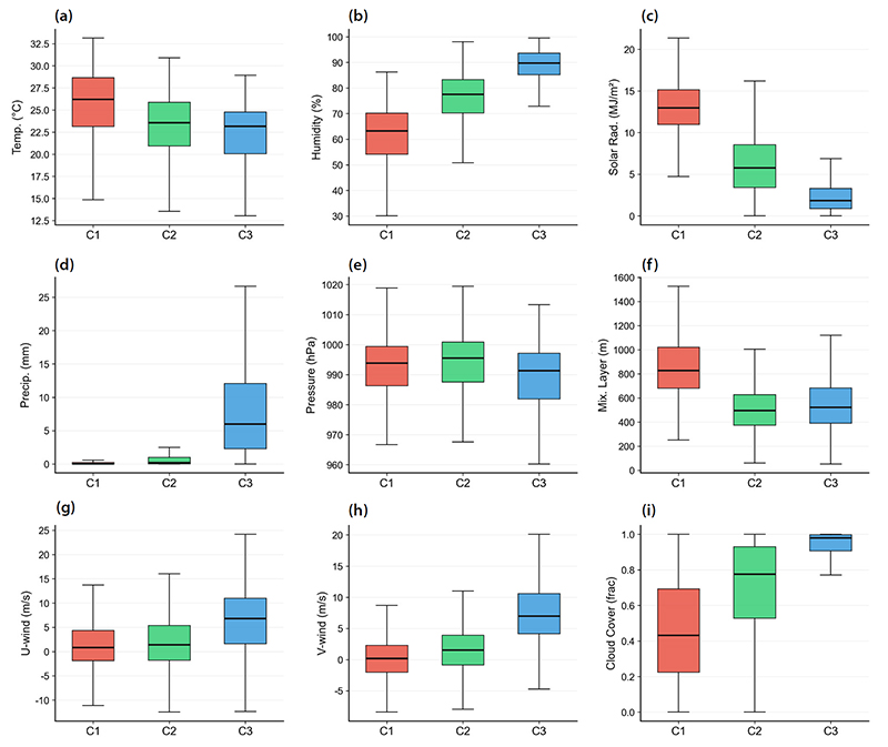
Distribution of nine ERA5 meteorological variables by cluster (C1, stagnant high-pressure; C2, low-radiation humid; C3, low-pressure precipitation): (a) temperature, (b) relative humidity, (c) solar radiation, (d) precipitation, (e) surface pressure, (f) planetary boundary layer height, (g) 850 hPa zonal wind, (h) 850 hPa meridional wind, (i) total cloud cover. Boxes indicate the interquartile range, horizontal lines indicate medians, and whiskers represent 1.5×IQR (outliers omitted for clarity).
군집별 월 구성을 살펴본 결과, 저기압 강수형(C3)은 7월(22.5%)과 8월(24.0%)의 비중이 5월(19.2%)·9월(16.9%)보다 뚜렷이 높아, 장마·태풍이 집중되는 시기와 강하게 연관되어 나타났다. 이는 군집화 입력 자료가 월별 평균을 차감한 편차임에도 불구하고, 저기압·강수를 동반하는 종관 기상 조건 자체가 특정 시기에 편중되어 발생하는 강한 신호를 반영하는 것으로 해석된다. 반면 정체 고기압형(C1)과 저일사 습윤형(C2)은 5~9월 전 기간에 걸쳐 19~21%의 비교적 균일한 비중을 보였는데, 이는 두 유형이 특정 월에 국한되지 않고 여름철 전반에 반복적으로 나타나는 배경 조건임을 보여준다(그림 2).
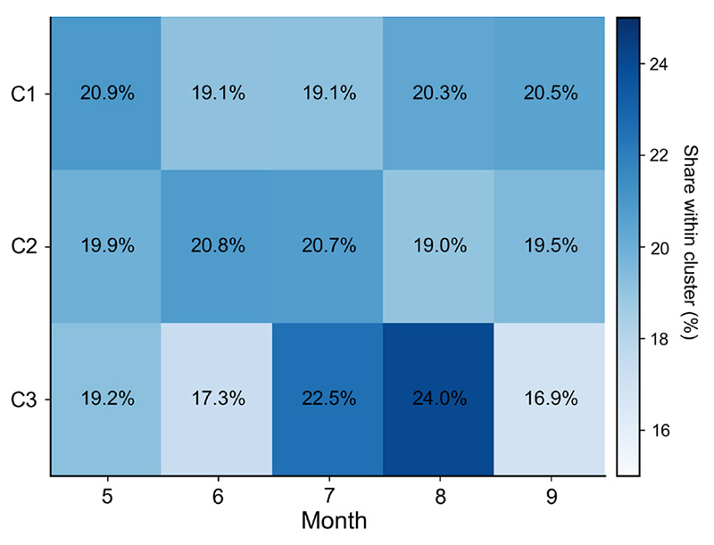
Monthly composition of each meteorological cluster (C1, stagnant high-pressure; C2, low-radiation humid; C3, low-pressure precipitation) during the study period (May~September, 2020~2024). Values indicate the percentage share of each month within a given cluster; rows sum to 100%.
군집별 MDA8 오존 농도를 비교한 결과(그림 3), 기상 유형에 따라 오존 농도 분포가 뚜렷하게 다르다(Kruskal-Wallis H=2060.3, p<0.001). MDA8 오존은 정체 고기압형(C1)에서 58.2±15.7 ppb로 가장 높았으며, 저일사 습윤형(C2) 50.1±14.4 ppb, 저기압 강수형(C3) 38.8±12.7 ppb 순으로 낮아졌다. 이는 맑고 정체된 고기압 환경에서 오존의 광화학적 생성이 촉진되는 반면, 강수 및 흐린 조건에서는 구름에 의한 일사 차단이 광화학적 오존 생성을 제한하는 메커니즘과 일치한다(Colombi et al., 2023; Bak et al., 2022). 특히 정체 고기압형(C1)은 사분위 범위(21.1 ppb)가 가장 넓고 최댓값도 141.0 ppb에 달해, 이 유형 내에서도 전구체 농도, 국지 기상 조건, 광화학 반응 간의 비선형 상호작용이 오존 변동성을 크게 좌우할 수 있음을 시사한다. 이러한 군집별 오존 농도 차이는 3개 기상 유형이 임의적인 통계적 분할이 아니라 실제 오존 농도 변동과 관련된 서로 다른 기상 조건을 반영함을 뒷받침하며, 전체 자료를 단일 모델로 분석할 경우 이러한 유형별 특성이 상쇄될 가능성을 시사한다.
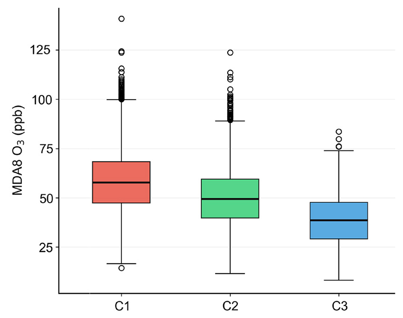
Distribution of MDA8 ozone concentrations by cluster (C1, stagnant high-pressure; C2, low-radiation humid; C3, low-pressure precipitation). Boxes indicate the interquartile range, horizontal lines indicate medians, whiskers represent 1.5×IQR, and points indicate outliers (Kruskal-Wallis H=2060.3, p<0.001).
3. 3 군집별 모델링 예측 성능
군집별 기상-오존 관계의 비선형성을 정량화하기 위해 군집별 독립 LightGBM 모델을 구축하고, 시간적 일반화 성능과 공간적 일반화 성능을 각각 LOYO 및 LORO 교차검증을 통해 평가하였다(그림 4). LOYO는 5개 연도를 순차적으로 제외하는 5-fold 방식으로 연도별 기상 조건 변동에 대한 예측 안정성을 평가하며(Stirnberg et al., 2021), LORO는 17개 시·도를 순차적으로 제외하는 17-fold 방식으로 미관측 지역에 대한 공간적 예측 가능성을 평가한다(Roberts et al., 2017).
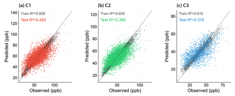
Observed versus predicted MDA8 O3 concentrations by cluster: (a) C1, stagnant high-pressure; (b) C2, low-radiation humid; (c) C3, low-pressure precipitation. Gray points indicate in-sample training predictions; colored points indicate out-of-sample Leave-One-Year-Out (LOYO) predictions. The dashed line indicates the 1 : 1 line.
트리 기반 앙상블 모델 4종(LightGBM, Random Forest, Gradient Boosting, XGBoost)의 LOYO 예측 성능을 비교한 결과, XGBoost(R2=0.506)가 근소하게 가장 높았으나 LightGBM (R2=0.500)과의 차이가 크지 않아 one-standard-error rule(Breiman et al., 1984) 에 따라 LightGBM을 최종 모델로 선정하였다. 모델별 상세 비교 결과는 표 S7에 제시하였다.
학습 R2는 정체 고기압형(C1)=0.938, 저일사 습윤형(C2)=0.935, 저기압 강수형(C3)=0.915로 모든 군집에서 높게 나타나, 각 유형 내 기상-오존 관계 구조를 모델이 잘 포착하고 있음을 보여준다. LOYO 검증 R2는 정체 고기압형(C1)=0.407, 저일사 습윤형(C2)=0.369, 저기압 강수형(C3)=0.360으로 나타났다. LOYO는 학습하지 않은 연도를 예측하는 구조이므로, 연도별 전구물질 배출량 변화·장거리 수송·지역별 배출 특성 등 기상변수로 포착되지 않는 비기상 요인이 오차로 직접 반영된다. 이 학습·검증 성능 격차(train-test gap)는 모델의 결함이 아니라 기상인자 단독 모델에서 구조적으로 예상되는 결과이며, 선행 연구의 유사 수준과도 일치한다(Colombi et al., 2023; Stirnberg et al., 2021). 높은 학습 R2는 각 유형 내에서 모델이 기상-오존 관계 구조를 충실하게 학습하였음을 보여준다. 군집 간 검증 성능 차이는 유형별로 기상-오존 관계가 나타나는 방식이 다르기 때문으로 해석된다. 정체 고기압형(C1, n=5,786)은 대기 정체와 높은 일사량이 비교적 일관되게 작용하는 유형으로 기상요인만으로도 오존 변동을 상대적으로 잘 설명할 수 있었던 반면, 저기압 강수형(C3, n=1,724)은 강수·일사량 감소·혼합층 변화·전구물질 농도 변화 등이 동시에 작용하여 기상인자만으로 오존 변동을 설명하는 데 상대적으로 큰 한계가 나타난 것으로 해석된다(Colombi et al., 2023; Bak et al., 2022).
군집별 모델의 성능을 해석하기 위한 기준으로, 군집 구분 없이 전체 13,005개 관측치에 단일 전역 모델을 별도로 구축하고 동일한 LOYO 절차로 평가하였다. 전역 모델의 검증 성능(LOYO R2=0.511)은 군집별 모델보다 높게 나타났는데, 이는 군집화에 따라 군집 내 오존 분산이 감소하여 결정계수 산정의 기준이 되는 총분산 자체가 작아졌기 때문으로 해석된다(표 S8). 본 연구는 예측 정확도보다 각 기상 유형에서 오존-기상 관계가 갖는 이질적 구조를 특성화하는 것을 목적으로 하므로(Molnar, 2022; Wu, 2022), 단일 전역 모델과의 성능 비교는 이러한 맥락에서 이해되어야 한다.
LORO 검증 결과, 세 유형 모두 LORO R2(정체 고기압형 0.459, 저일사 습윤형 0.474, 저기압 강수형 0.485) 가 LOYO R2보다 높게 나타나, 공간적 일반화가 시간적 일반화보다 상대적으로 용이한 것으로 나타났다(표 S5). 다만 LOYO는 5개 연도, LORO는 17개 지역을 기준으로 폴드를 구성하여 학습:검증 자료 비율이 서로 달라(약 4:1 대 16:1), 두 결과의 직접적 비교에는 이러한 폴드 구성 차이를 감안할 필요가 있다. 이는 세 기상 유형이 특정 지역에 국한되지 않고 여러 지역에서 공통적으로 나타나는 종관 규모의 기상 조건을 반영하며, 반면 연도 간 차이는 기상변수로 포착되지 않는 배출량 변화 등 비기상요인의 영향을 상대적으로 크게 받기 때문으로 해석된다(Grange et al., 2018). 지역별 상세 결과는 표 S9에 제시하였다. LOYO 폴드 간 변수 중요도 순위의 스피어만 상관계수는 정체 고기압형(C1) r=0.96, 저일사 습윤형(C2) r=0.91, 저기압 강수형(C3) r=0.94로 나타나, 표본 수가 상대적으로 적은 저기압 강수형(C3)을 포함하여 세 유형 모두에서 연도 간 높은 재현성이 확인되었다(그림 S3).
3. 4 기상변수의 오존 기여 메커니즘 분석
그림 5는 군집별 SHAP beeswarm 도표 결과를 나타낸 것이다. 이때 제시된 SHAP 중요도는 각 군집 내부에서 산출된 조건부 기여도로, 군집 구분 자체에 사용된 변수의 중요도와는 구분된다. 정체 고기압형(C1)은 상대습도의 mean |SHAP|가 6.90 ppb로 가장 높았으며, 기온(2.92 ppb)과 850 hPa 동서 방향 바람 성분(2.59 ppb)이 뒤를 이었다. 이는 대기 중 수증기가 오존 광분해로 생성된 여기상태 산소원자와 반응하여 OH 라디칼을 생성함으로써, 오존의 광화학적 소멸 및 생성 효율에 직접 관여하는 독립적 화학인자로 작용하기 때문으로 해석된다(Porter and Heald, 2019). 동서 방향 바람 성분의 중요도는 대기가 전반적으로 정체된 상태에서도 미세한 풍향 변화가 유입 기단의 기원과 전구물질의 국지적 축적 정도에 영향을 줄 수 있음을 시사하며, 혼합층고도(2.32 ppb) 역시 4순위로 나타나 연직 확산 조건의 변동이 오존 농도에 부가적으로 기여한 것으로 해석된다.
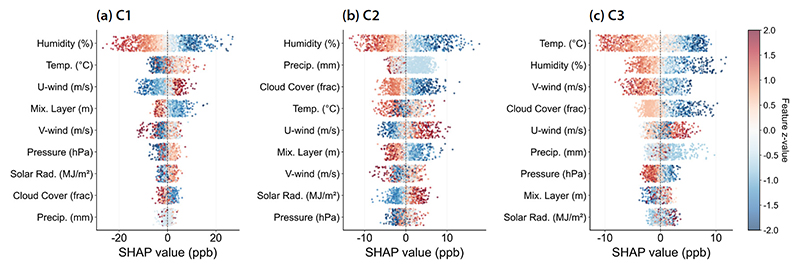
SHAP beeswarm plots of feature contributions to MDA8 O3 predictions by cluster: (a) C1, stagnant high-pressure; (b) C2, low-radiation humid; (c) C3, low-pressure precipitation. Features are ranked by mean absolute SHAP value (top=most important). Point color indicates the standardized (z-score) value of each feature; horizontal position indicates the SHAP value (ppb).
저일사 습윤형(C2)에서도 상대습도(4.02 ppb)가 가장 높았으며, 강수량(2.43 ppb)과 전운량(2.13 ppb)이 기온(1.74 ppb)보다 높은 중요도를 보여 구름·강수에 따른 오존 생성 억제 효과를 반영하는 것으로 해석된다. 850 hPa 동서 방향 바람 성분(1.73 ppb)은 기온과 비슷한 수준의 중요도를 보여, 흐리고 습윤한 조건에서도 하층 바람에 의한 수증기·오염물질 이류가 오존 변동에 일부 기여하는 것으로 판단된다.
저기압 강수형(C3)에서는 기온(4.36 ppb)의 mean |SHAP|가 가장 높았고 상대습도(2.21 ppb)와 850 hPa 남북 방향 바람 성분(1.95 ppb)이 뒤를 이었다. 남북 방향 바람 성분의 높은 중요도는 저기압·전선 통과에 수반되는 남풍·북풍 전환이 기단 교체 및 수증기 유입 경로 변화와 연관됨을 시사한다. 반면 지표기압의 중요도는 0.86 ppb로 상대적으로 낮았는데, 이는 이 유형이 이미 낮은 기압(989.1 hPa 내외)으로 정의되어 군집 내부에서 기압 자체의 변동 폭이 작기 때문으로 해석된다. 일사량 역시 0.68 ppb로 9개 변수 중 가장 낮았으며, 같은 이유로 이 유형 내에서 이미 제한된 범위를 가지므로 설명력이 낮게 나타난 것으로 판단된다.
군집별로 기온-SHAP 관계의 비선형 구조는 뚜렷하게 다르게 나타났다(그림 6). 정체 고기압형(C1)과 저일사 습윤형(C2)에서는 공통적으로 기온 상승에 따라 SHAP 값이 증가하다가 특정 온도(각각 약 26°C, 24°C) 이후 정체되거나 감소하는 역U자형 패턴이 나타났다. 이 전환 구간은 고온 조건이 구름 증가·일사 차단을 동반하는 시기와 관련될 수 있으며, 고온 구간에서 양의 기여가 약화되는 현상은 기온 자체의 효과가 역전된 것이 아니라 고온에 수반되는 복합 기상 조건이 오존의 광화학적 생성을 부분적으로 제한한 결과로 해석된다(Colombi et al., 2023; Bak et al., 2022). 다만 저일사 습윤형(C2)의 고온 구간 감소 폭이 정체 고기압형(C1)보다 더 급격하게 나타나, 이미 흐리고 습윤한 배경 조건에서는 고온이 동반하는 억제 효과가 상대적으로 크게 작용하는 것으로 보인다.
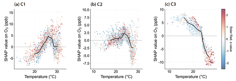
SHAP dependence plots for temperature by cluster: (a) C1, stagnant high-pressure; (b) C2, low-radiation humid; (c) C3, low-pressure precipitation. Point color indicates the standardized (z-score) value of solar radiation; the black line indicates the binned mean SHAP value.
반면 저기압 강수형(C3)에서는 역U자형이 아니라, 관측된 온도 범위(약 16~27°C) 전 구간에서 SHAP 값이 지속적으로 감소하는 단조 감소 패턴이 나타났다. 이는 이 유형의 관측치가 애초에 저기압·강수와 결부된 서늘한 조건에 상대적으로 집중되어 있어, 기온이 낮을수록 강한 양의 기여를 보이고 기온이 높아질수록 강수·구름 조건에서 벗어나며 기여가 급격히 감소하는 것으로 해석된다.
그림 7의 색상 분포에서, 정체 고기압형(C1)과 저일사 습윤형(C2)에서는 고온 관측치(붉은 점)가 양의 SHAP 영역에 상대적으로 많이 분포하여 기온과 일사량의 결합 효과가 MDA8 오존 예측에 반영되었음을 보여준다(Lundberg and Lee, 2017). 일사량의 군집별 비선형 반응을 보면, 정체 고기압형(C1)에서는 일사량 증가에 따라 SHAP 값이 상승하다 약 14~15 MJ m-2 이후 정체되는 완만한 역U자형을 보였고, 저일사 습윤형(C2)에서는 관측 범위가 좁게 제한되는 가운데 단조 증가 경향이 유지되었다. 반면 저기압 강수형(C3)에서는 일사량 자체가 좁은 범위(0~6 MJ m-2 내외)에 국한되어 있어 뚜렷한 추세 없이 SHAP 값이 0 부근에서 등락하는 양상을 보였는데, 이는 이 유형에서 일사량의 mean |SHAP|가 9개 변수 중 가장 낮았던 결과와도 일치한다.
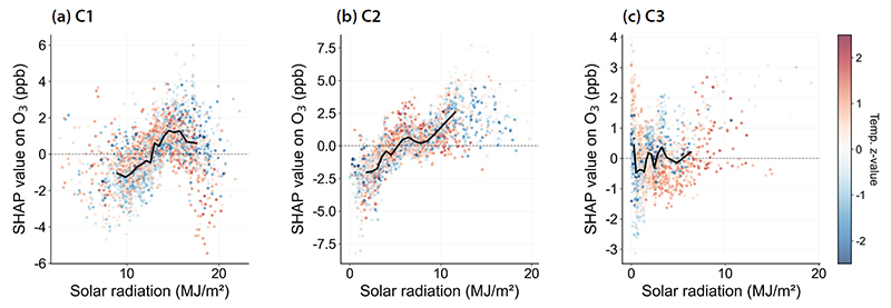
SHAP dependence plots for solar radiation by cluster: (a) C1, stagnant high-pressure; (b) C2, low-radiation humid; (c) C3, low-pressure precipitation. Point color indicates the standardized (z-score) value of temperature; the black line indicates the binned mean SHAP value.
4. 결 론
본 연구는 2020~2024년 5~9월 전국 17개 시·도의 일별 MDA8 오존 및 ERA5 기상 자료(13,005개 관측치)를 대상으로, K-평균 기반 기상 유형 군집화와 군집별 LightGBM-SHAP 분석을 수행하여 오존-기상 관계의 유형별 이질성을 규명하였다.
(1) K-평균 군집화 결과 3개의 기상 유형(정체 고기압형 C1, 44.5%; 저일사 습윤형 C2, 42.3%; 저기압 강수형 C3, 13.3%)이 도출되었으며, Bootstrap ARI=0.893으로 안정성이 확인되었다.
(2) MDA8 오존 평균 농도는 정체 고기압형(58.2 ppb)>저일사 습윤형(50.1 ppb)>저기압 강수형(38.8 ppb) 순으로 유의하게 달랐다(Kruskal-Wallis, p<0.001). 정체 고기압형은 대기 정체·높은 일사량·낮은 강수량이, 저기압 강수형은 강수·운량 증가에 따른 일사 제한이 이러한 차이를 설명한다.
(3) 군집별 LightGBM 모델의 LOYO 검증 R2는 정체 고기압형(0.407)>저일사 습윤형(0.369)>저기압 강수형(0.360) 순이었다. 이는 단일 전역 모델(R2=0.511)보다 낮은 값이나, 이는 군집화로 군집 내 오존 분산이 감소하여 R2 산정 기준이 되는 총분산 자체가 작아졌기 때문이다. 실제로 군집별 모델의 표본크기 가중 평균 RMSE는 11.42 ppb로 전역 모델(11.30 ppb)과 1% 이내로 유사하며, 이를 전역 분산 기준으로 환산하면 R2 ~0.50 수준으로 전역 모델과 사실상 동등하다. 즉 군집별 모델은 예측 성능을 잃지 않으면서도 유형별 해석 해상도를 확보하였다는 점에서 의의가 있다.
(4) SHAP 분석 결과 정체 고기압형·저일사 습윤형에서는 상대습도가, 저기압 강수형에서는 기온이 가장 중요한 변수로 확인되어, 군집을 정의하는 배경 조건과 내부 설명변수가 다를 수 있음을 보여주었다. 기온-오존 관계의 비선형 구조 역시 유형별로 달랐다(정체 고기압형·저일사 습윤형의 역U자형, 저기압 강수형의 단조 감소).
본 연구는 지역·계절을 사전에 고정하지 않고 기상 조건에 기반해 유형을 식별함으로써, 단일 모델에서는 가려질 수 있는 오존-기상 관계의 유형별 이질성을 드러냈다는 점에서 의의가 있다.
다만 기상변수만을 사용하여 전구물질(NOx, VOCs) 배출량과 장거리 수송의 영향은 반영하지 못하였다. 오존 생성은 NOx·VOCs 비율에 따라 민감도가 달라지므로, 향후 전구물질 자료를 함께 활용하면 오존 생성 메커니즘을 더 정교하게 규명하고 저감 전략 수립에도 근거를 제공할 수 있을 것이다. 일별 자료의 한계상 고해상도 시간 자료를 결합한 후속 연구도 필요하다.
Acknowledgments
본 논문은 2026년도 교육부 및 전라남도의 재원으로 전라남도RISE센터의 지원을 받아 수행된 지역혁신중심 대학지원체계 (RISE)의 결과입니다 (2026-RISE-14-007). 또한 본 연구와 관련하여 (주)송림의 기술적 자문과 협조에 감사드립니다.
References
-
Bak, J., Song, E.-J., Lee, H.-J., Liu, X., Koo, J.-H., Kim, J., Jeon, W., Kim, J.-H., Kim, C.-H. (2022) Temporal variability of tropospheric ozone and ozone profiles in the Korean Peninsula during the East Asian summer monsoon: Insights from multiple measurements and reanalysis datasets, Atmospheric Chemistry and Physics, 22, 14177-14187.
[https://doi.org/10.5194/acp-22-14177-2022]

-
Balogun, A.-L. Tella, A. (2022) Modelling and investigating the impacts of climatic variables on ozone concentration in Malaysia using correlation analysis with random forest, decision tree regression, linear regression, and support vector regression, Chemosphere, 299, 134250.
[https://doi.org/10.1016/j.chemosphere.2022.134250]
-
Breiman, L. (2001) Random forests, Machine Learning, 45(1), 5-32.
[https://doi.org/10.1023/A:1010933404324]
- Breiman, L., Friedman, J.H., Olshen, R.A., Stone, C.J. (1984) Classification and Regression Trees, Wadsworth, Belmont, CA, USA.
-
Chai, T., Draxler, R.R. (2014) Root mean square error (RMSE) or mean absolute error (MAE)? - Arguments against avoiding RMSE in the literature, Geoscientific Model Development, 7(3), 1247-1250.
[https://doi.org/10.5194/gmd-7-1247-2014]
-
Colombi, N.K., Jacob, D.J., Yang, L.H., Zhai, S., Shah, V., Grange, S.K., Yantosca, R.M., Kim, S., Liao, H. (2023) Why is ozone in South Korea and the Seoul metropolitan area so high and increasing?, Atmospheric Chemistry and Physics, 23(7), 4031-4044.
[https://doi.org/10.5194/acp-23-4031-2023]
-
Grange, S.K., Carslaw, D.C., Lewis, A.C., Boleti, E., Hueglin, C. (2018) Random forest meteorological normalisation models for Swiss PM10 trend analysis, Atmospheric Chemistry and Physics, 18(9), 6223-6239.
[https://doi.org/10.5194/acp-18-6223-2018]
-
Guan, Y., Xiao, Y., Chu, C., Zhang, N., Yu, L. (2022) Trends and characteristics of ozone and nitrogen dioxide related health impacts in Chinese cities, Ecotoxicology and Environmental Safety, 241, 113808.
[https://doi.org/10.1016/j.ecoenv.2022.113808]
-
Hastie, T., Tibshirani, R., Friedman, J. (2009) The Elements of Statistical Learning: Data Mining, Inference, and Prediction, 2nd ed., Springer, New York, USA.
[https://doi.org/10.1007/978-0-387-84858-7]
-
Hersbach, H., Bell, B., Berrisford, P., Hirahara, S., Horányi, A., Muñoz-Sabater, J., Nicolas, J., Peubey, C., Radu, R., Schepers, D., Simmons, A., Soci, C., Abdalla, S., Abellan, X., Balsamo, G., Bechtold, P., Biavati, G., Bidlot, J., Bonavita, M., De Chiara, G., Dahlgren, P., Dee, D., Diamantakis, M., Dragani, R., Flemming, J., Forbes, R., Fuentes, M., Geer, A., Haimberger, L., Healy, S., Hogan, R.J., Hólm, E., Janisková, M., Keeley, S., Laloyaux, P., Lopez, P., Lupu, C., Radnoti, G., de Rosnay, P., Rozum, I., Vamborg, F., Villaume, S., Thépaut, J.-N. (2020) The ERA5 global reanalysis, Quarterly Journal of the Royal Meteorological Society, 146(730), 1999-2049.
[https://doi.org/10.1002/qj.3803]
-
Houdou, A., El Badisy, I., Khomsi, K., Abdala, S.A., Abdulla, F., Najmi, H., Obtel, M., Belyamani, L., Ibrahimi, A., Khalis, M. (2024) Interpretable machine learning approaches for forecasting and predicting air pollution: A systematic review, Aerosol and Air Quality Research, 24, 230151.
[https://doi.org/10.4209/aaqr.230151]
-
Hubert, L., Arabie, P. (1985) Comparing partitions, Journal of Classification, 2(1), 193-218.
[https://doi.org/10.1007/BF01908075]
-
Iungman, T., Khomenko, S., Barboza, E.P., Cirach, M., Gonçalves, K., Petrone, P., Erbertseder, T., Taubenböck, H., Chakraborty, T., Nieuwenhuijsen, M. (2024) The impact of urban configuration types on urban heat islands, air pollution, CO2 emissions, and mortality in Europe: A data science approach, The Lancet Planetary Health, 8(7), e489-e505.
[https://doi.org/10.1016/S2542-5196(24)00120-7]
-
Jung, M.-W., Lee, J.-Y., Wang, K.-H., Lee, C.-Y., Han, S.-H., Kim, H.-J., Sohn, S.-M., Jeong, P.-S., Choi, D.-R., Yun, H.-Y. (2025) Development of a Conv-LSTM-Based AI Model for Forecasting PM2.5 Spatial Concentration Distribution, Journal of Korean Society for Atmospheric Environment, 41(1), 67-82, (in Korean with English abstract).
[https://doi.org/10.5572/KOSAE.2025.41.1.067]
- Ke, G., Meng, Q., Finley, T., Wang, T., Chen, W., Ma, W., Ye, Q., Liu, T.-Y. (2017) LightGBM: A highly efficient gradient boosting decision tree, Advances in Neural Information Processing Systems, 30, 3146-3154. https://papers.neurips.cc/paper/2017/hash/6449f44a102fde848669bdd9eb6b76fa-Abstract.html
-
Kim, J., Choi, M., Jeon, Y., Kim, T., Kwak, K.-H., Lee, G., Kang, B., Jung, S. (2025) Enhancing the Simulation Performance of PM2.5 Compositions in the WRF-CMAQ Modeling System Using Machine Learning Techniques, Journal of Korean Society for Atmospheric Environment, 41(3), 430-447, (in Korean with English abstract).
[https://doi.org/10.5572/KOSAE.2025.41.3.430]
-
Lee, H., Park, R., Jeong, J. (2024) Impact of Recent Meteorological Changes on Surface Ozone Increases in Seoul Metropolitan Area, Journal of Korean Society for Atmospheric Environment, 40(4), 467-476, (in Korean with English abstract).
[https://doi.org/10.5572/KOSAE.2024.40.4.467]
-
Lee, K.-H., Lee, K.-T. (2020) Characteristics of Atmospheric Aerosols Based on Column Measurements by Using Machine Learning Clustering, Journal of Korean Society for Atmospheric Environment, 36(5), 608-619, (in Korean with English abstract).
[https://doi.org/10.5572/KOSAE.2020.36.5.608]
-
Liu, N., He, G., Wang, H., He, C., Wang, H., Liu, C., Wang, Y., Wang, H., Li, L., Lu, X., Fan, S. (2023) Rising frequency of ozone-favorable synoptic weather patterns contributes to 2015-2022 ozone increase in Guangzhou, Journal of Environmental Sciences, 148, 502-514.
[https://doi.org/10.1016/j.jes.2023.09.024]
-
Lloyd, S.P. (1982) Least squares quantization in PCM, IEEE Transactions on Information Theory, 28(2), 129-137.
[https://doi.org/10.1109/TIT.1982.1056489]
- Lundberg, S.M., Lee, S.-I. (2017) A unified approach to interpreting model predictions, Advances in Neural Information Processing Systems, 30, 4765-4774. https://papers.neurips.cc/paper/2017/hash/8a20a8621978632d76c43dfd28b67767-Abstract.html
-
Lundberg, S.M., Erion, G., Chen, H., DeGrave, A., Prutkin, J.M., Nair, B., Katz, R., Himmelfarb, J., Bansal, N., Lee, S.-I. (2020) From local explanations to global understanding with explainable AI for trees, Nature Machine Intelligence, 2(1), 56-67.
[https://doi.org/10.1038/s42256-019-0138-9]
-
McInnes, L., Healy, J., Melville, J. (2018) UMAP: Uniform manifold approximation and projection for dimension reduction, Journal of Open Source Software, 3(29), 861.
[https://doi.org/10.21105/joss.00861]
-
Méndez, M., Merayo, M.G., Nuñez, M. (2023) Machine learning algorithms to forecast air quality: A survey, Artificial Intelligence Review, 56, 10031-10066.
[https://doi.org/10.1007/s10462-023-10424-4]
- Molnar, C. (2022) Interpretable Machine Learning: A Guide for Making Black Box Models Explainable, 2nd ed., Leanpub, Victoria, Canada. https://christophm.github.io/interpretable-ml-book/
-
Oak, Y.J., Jacob, D.J., Pendergrass, D.C., Dang, R., Colombi, N.K., Chong, H., Lee, S., Kuk, S.K., Kim, J. (2025) Air quality trends and regimes in South Korea inferred from 2015-2023 surface and satellite observations, Atmospheric Chemistry and Physics, 25, 3233-3252.
[https://doi.org/10.5194/acp-25-3233-2025]
-
Park, J.-S., Song, Y.-J., Suh, M.-S., Kim, C. (2023) Prediction of PM2.5 using Super Learner Ensemble, Journal of Korean Society for Atmospheric Environment, 39(6), 1038-1049, (in Korean with English abstract).
[https://doi.org/10.5572/KOSAE.2023.39.6.1038]
-
Porter, W.C., Heald, C.L. (2019) The mechanisms and meteorological drivers of the summertime ozone-temperature relationship, Atmospheric Chemistry and Physics, 19(21), 13367-13381.
[https://doi.org/10.5194/acp-19-13367-2019]
-
Qiu, M., Zigler, C., Selin, N.E. (2022) Statistical and machine learning methods for evaluating trends in air quality under changing meteorological conditions, Atmospheric Chemistry and Physics, 22, 10551-10566.
[https://doi.org/10.5194/acp-22-10551-2022]
-
Reddy, B.S.K., Kumar, K.R., Balakrishnaiah, G., Gopal, K.R., Reddy, R.R., Sivakumar, V., Lingaswamy, A.P., Arafath, S.M., Umadevi, K., Kumari, S.P., Ahammed, Y.N., Lal, S. (2012) Analysis of diurnal and seasonal behavior of surface ozone and its precursors (NOx) at a semi-arid rural site in southern India, Aerosol and Air Quality Research, 12(6), 1081-1094.
[https://doi.org/10.4209/aaqr.2012.03.0055]
-
Roberts, D.R., Bahn, V., Ciuti, S., Boyce, M.S., Elith, J., Guillera-Arroita, G., Hauenstein, S., Lahoz-Monfort, J.J., Schröder, B., Thuiller, W., Warton, D.I., Wintle, B.A., Hartig, F., Dormann, C.F. (2017) Cross-validation strategies for data with temporal, spatial, hierarchical, or phylogenetic structure, Ecography, 40(8), 913-929.
[https://doi.org/10.1111/ecog.02881]
-
Rousseeuw, P.J. (1987) Silhouettes: A graphical aid to the interpretation and validation of cluster analysis, Journal of Computational and Applied Mathematics, 20, 53-65.
[https://doi.org/10.1016/0377-0427(87)90125-7]
-
Seo, J., Youn, D., Kim, J.Y., Lee, H. (2014) Extensive spatiotemporal analyses of surface ozone and related meteorological variables in South Korea for the period 1999-2010, Atmospheric Chemistry and Physics, 14(12), 6395-6415.
[https://doi.org/10.5194/acp-14-6395-2014]
-
Son, M., Kim, J. (2023) Digital transformation of rotary hearth furnace for process automation and CO2 reduction: Hybrid model under limited operational data utilization, Journal of Manufacturing Processes, 101, 784-794.
[https://doi.org/10.1016/j.jmapro.2023.05.108]
-
Stirnberg, R., Cermak, J., Kotthaus, S., Haeffelin, M., Andersen, H., Fuchs, J., Kim, M., Petit, J.-E., Favez, O. (2021) Meteorology-driven variability of air pollution (PM1) revealed with explainable machine learning, Atmospheric Chemistry and Physics, 21(5), 3919-3948.
[https://doi.org/10.5194/acp-21-3919-2021]
- World Health Organization (WHO) (2021) WHO global air quality guidelines: Particulate matter (PM2.5 and PM10), ozone, nitrogen dioxide, sulfur dioxide and carbon monoxide, World Health Organization, Geneva, Switzerland. https://iris.who.int/handle/10665/345329
-
Wu, J., Chen, X., Li, R., Wang, A., Huang, S., Li, Q., Qi, H., Liu, M., Cheng, H., Wang, Z. (2024) A novel framework for high resolution air quality index prediction with interpretable artificial intelligence and uncertainties estimation, Journal of Environmental Management, 357, 120785.
[https://doi.org/10.1016/j.jenvman.2024.120785]
-
Wu, X. (2022) Tri-clustering-based exploration of spatio-temporal heterogeneity of six criteria air pollutants and their relationships in China, Frontiers in Earth Science, 10, 951510.
[https://doi.org/10.3389/feart.2022.951510]
-
Ye, X., Zhang, L., Wang, X., Lu, N., Hickman, S., Luo, G., Archibald, A.T. (2026) Deciphering the impacts of meteorology on surface ozone variability in eastern China using explainable machine learning models, Atmospheric Chemistry and Physics, 26, 6377-6390.
[https://doi.org/10.5194/acp-26-6377-2026]
-
Yeo, J., Kim, B.-U. (2022) Long-term trend analysis of ozone and PM2.5 in South Korea and attribution to meteorological and emission changes, Atmospheric Environment, 272, 118942.
[https://doi.org/10.1016/j.atmosenv.2022.118942]
-
Zhan, C., Xie, M., Lu, H., Liu, B., Wu, Z., Wang, T., Zhuang, B., Li, M., Li, S. (2023) Impacts of urbanization on air quality and the related health risks in a city with complex terrain, Atmospheric Chemistry and Physics, 23, 771-788.
[https://doi.org/10.5194/acp-23-771-2023]
Appendix
Supplementary Materials
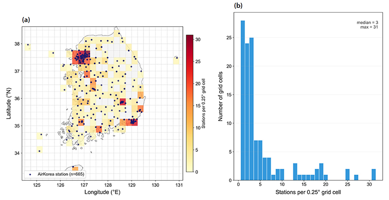
Spatial correspondence between AirKorea monitoring stations and the ERA5 0.25° grid. (a) Locations of the 665 stations used in the analysis (dark points) over the South Korean coastline, overlaid on a 0.25° grid (dashed lines) shaded by the number of stations mapped to each cell. (b) Histogram of the number of stations per occupied grid cell (median=3, maximum=31, at a cell in central Seoul).
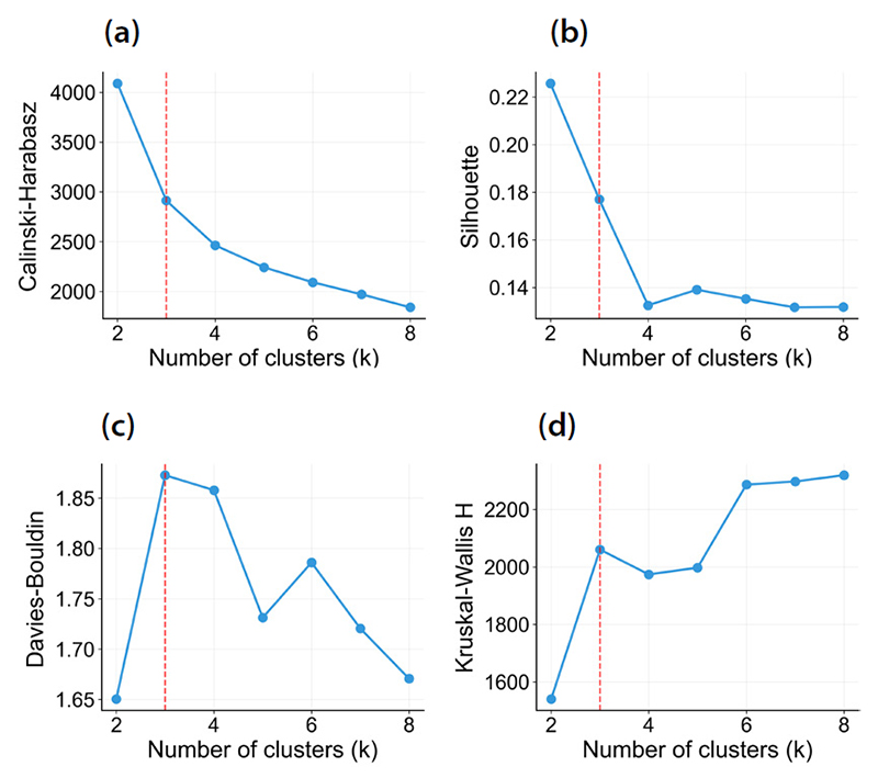
Clustering evaluation metrics across candidate numbers of clusters (k=2~8): (a) Calinski-Harabasz index, (b) Silhouette coefficient, (c) Davies-Bouldin index, (d) Kruskal-Wallis H statistic for MDA8 O3. The vertical dashed line indicates the selected k=3.
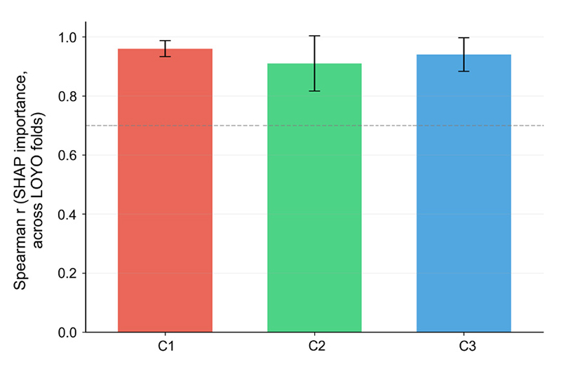
Reproducibility of SHAP-based variable importance rankings across Leave-One-Year-Out (LOYO) folds, expressed as the mean Spearman rank correlation (bars) with the range down to the minimum observed correlation (error bars) for each cluster (C1, stagnant high-pressure; C2, low-radiation humid; C3, low-pressure precipitation).
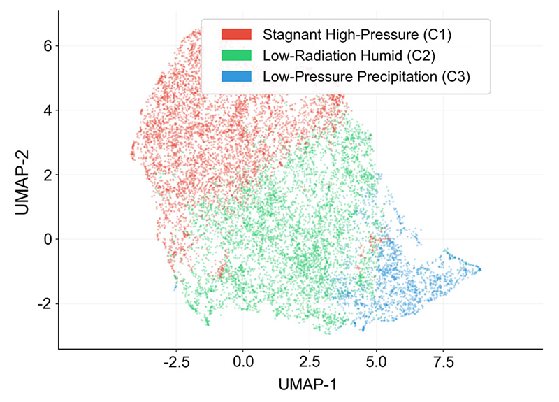
UMAP projection of nine-dimensional standardized monthly ERA5 meteorological anomalies, colored by K-means cluster assignment (C1, stagnant high-pressure; C2, low-radiation humid; C3, low-pressure precipitation). UMAP was used for visualization only and was not involved in the clustering procedure (n_neighbors=15, min_dist=0.1).
Variable-level agreement between station-weighted daily regional means (current method) and grid-weighted means (removing duplicate weighting from densely monitored cells), for all nine meteorological variables: Pearson correlation, mean absolute difference (MAD), and MAD/SD.
Agreement between K-means (k=3) cluster labels derived from the station-weighted and grid-weighted meteorological aggregation schemes described in Table S1, summarized as the Adjusted Rand Index and the identical-assignment rate across all 13,005 sido-day observations.
Bootstrap Adjusted Rand Index (ARI) for candidate numbers of clusters (k= ~4), assessing the stability of K-means cluster assignments under resampling.
Optimal LightGBM hyperparameters for each cluster, selected via 5-fold grid search cross-validation minimizing validation RMSE.
Cluster-specific model performance (R2, RMSE, MAE) under Leave-One-Year-Out (LOYO) and Leave-One-Region-Out (LORO) cross-validation, along with training performance and the single global model’s LOYO R2.
Mean absolute SHAP values for all nine ERA5 meteorological variables, by cluster.
Leave-One-Year-Out (LOYO) predictive performance of four tree-based ensemble models (LightGBM, Random Forest, Gradient Boosting, XGBoost).
Comparison of predictive performance (LOYO R2, RMSE, MAE) between the single global model and the three cluster-specific models.
Cluster-specific and mean Leave-One-Region-Out (LORO) R2 and RMSE by metropolitan region, sorted by mean R2 in descending order.
정선기(전남대학교 환경시스템공학과 학석연계과정 학생, jsk659@jnu.ac.kr) Methodology, Software, Investigation, Data curation, Visualization, Writing - original draft
정준영(전남대학교 건설·환경공학과 석사과정 학생, jjy01124@jnu.ac.kr) Software, Formal analysis, Validation
최아름(전남대학교 환경시스템공학과 연구원, shaina0218@jnu.ac.kr) Data curation, Investigation, Validation
김진수(건국대학교 화공생명에너지공학과 조교수, jkim1102@konkuk.ac.kr) Conceptualization, Methodology, Writing - review & editing, Supervision
장지이(전남대학교 환경시스템공학과 조교수, jiyi.jang@jnu.ac.kr) Conceptualization, Writing - review & editing, Supervision, Project administration, Funding acquisition